jngannon.github.io
Blog
Pruning, cost functions and adversarial noise.
Introduction
This article and the attached notebooks demonstrate potential advantages of removing the softmax from the final layer of a neural network and pruning weights based on their activated value, and absolute value. Using a model with less weights can potentially run faster. An interesting result is improved performance with regard to adversarial noise. I assume a working knowledge of neural networks and adversarial noise. A complete list of adversarial defences and attacks can be found here https://www.robust-ml.org/. I have not included any mathematical equations in these blogs, just descriptions, they are all widely used methods, and the code is available for anyone looking verify. The notebooks used are available, however running these as they are may result in different results. Different models can be loaded, and different hyperparameters used.
Definitions
For the sake of clarity, there are some terms that i use often here that I will define clearly.
Activated value: The value of weights multiplied by their input. These experiments use the mean of the values taken from 2000 inputs. Algorithm described in more detail below.
Absolute value: The absolute value of weights, no input required.
Robustness: Real accuracy with adversarial noise added.
Resiliance: able to be pruned without losing test accuracy performance.
Pruning: Setting the value of weights in a weight matrix to 0.
Linear-quadratic model: Model trained with no softmax function, final layer outputs used directly with quadratic cost function.
Softmax-cross entropy model: Model trained with the softmax function applied to the final layer with cross entropy cost function.
Models used
I will demonstrate parameter pruning on both a convolutional neural network(CNN), and a fully connected neural network(ANN). The CNN gets better overall performance, but is slow to work with for demonstration purposes. Using a smaller ANN that trains and runs faster allows me to run many more tests, and get enough data to make plots to demonstrate things.
ANN
4 layer fully connected neural network 3 fully connected layers with 1500, 1000, and 800 neurons with ReLu activations, and an output layer. Trained with tensorflow ADAM optimizer, using quadratic cost, and L2 regularization, and a dropout rate of 0.7. The model is trained for 100,000 iterations with a mini-batch of 250 datapoints. The training time might seem like overkill, a similar overall performance can be achieved with 10,000 iterations, the reasons are explained later.
CNN
7 layer network with 4 convolutional layers, 2 fully connected layer all with ReLu activations, and an output layer. Trained with tensorflow ADAM optimizer, using quadratic cost, and L2 regularization, and dropout rate of 0.7. To prune, i have decoupled convolutional layers into sparse, fully connected layers, then pruned as if the weights were then independent.
Lose the softmax
I have removed the softmax from the final layer of both models demonstrated here. The cost is simple quadratic cost with L2 regulaization applied directly to the outputs of the final layer. I refer to these models as linear-quadratic models. I have found small increases in performance to begin with, but they may well be within what is reasonably expected from random initialization. I found it much more difficult to train adversarial noise with linear outputs and a quadratic cost. A softmax function can be applies to an already trained model, and the cost function replaced with cross entropy to generate adversarial noise that corrupts the model in the same way. The next article on output analysis has more detail.
Activated values
The algorithm is:
- Initialize a ‘mean activated values’ matrix of zeros the same size as the weight matrix.
- Multiply the weight matrix by the corresponding input vector, in tensorflow I use tf.multiply(weight_matrix, tf.transpose(input_vector)).
- Add the activated weights to the ‘mean activated values’ matrix.
- Repeat 2 and 3 for the required number of data points.
- Divide the ‘mean activated values’ matrix by the number of samples.
For these experiments I have used 2000 randomly selected images from the test set.
Generating noise
The code that I refered to to generate the adversarial noise is found here: https://github.com/Hvass-Labs/TensorFlow-Tutorials Notebooks 11 and 12 are tutorials about generating adversarial noise. They are very clear, thorough, and very well commented. The notebook that I have attached is not intended to be a tutorial, the same method is used to generate the noise.
I could not generate noise using linear outputs and a quadratic cost funciton that would effectively corrupt images enough to test on. I added a softmax function and replaced the cost function with cross entropy on an already trained model, and generated the noise vectors. I also found that noise generated on a softmax-cross entropy model with the same architecture also corrupted images, although to a lesser extent.
The notebook I used is called Make_Some_Noise, but if anyone is interested in how it works, read the link above, and the other stuff from Hvass-Labs, it is very well written.
Pruning for speed
Pruning models can potentially have a speed advantage, but i have developed these models using tensorflow, which is not optimized to run sparse matrix operations on gpu, so I can’t do the best comparison using this platform.
To prune the convolutional neural network I have ‘decoupled’ the convolutional layers into fully connected layers after being trained. These matrices are too big to fit into memory, so i have comverted them into scipy sparse arrays. ‘Decoupling the convolutional layers just involves converting each time a filter is applied to a row of a weight matrix. The speed of matrix multiplication in sparse arrays is directly proportional to the number of entries, so pruning has a real speed advantage. I have only run this using the python @ operator, which runs on a single thread for sparse arrays. There is a speed advantage to models with less parameters, but until i am using optimized code, the numbers are not very useful.
Pruning for security
The use of neural networks is growing rapidly, but the problem of adversarial noise has not been solved. The problem is more complicated than it initially seems, and the best solution will probably turn out to be a combination of strategies.
Below are a few methods of deciding which parameters to prune from fully connected neural networks. Different noise vectors are added to try and evaluate robustness with respect to different classes and intensities. It is interesting to note how different noise vectors behave differently. This is a demonstration of the complexity of the problem. The limit refered to in the plots is the limit on pixel intensity. While it may seem like best practice to test on the most successful attack, the selection of noise vectors is intended to show that the trend of increased robustness holds for vectors of higher and lower pixel intensity, and higher and lower corrupting effectiveness.
Absolute Values
The plot below shows a 4 layer fully connected neural network pruned based on the smallest absolute value. The following plots only show a selection of noise vectors that i have created, this is to keep the plots more readable, while giving an idea of the overall trend.
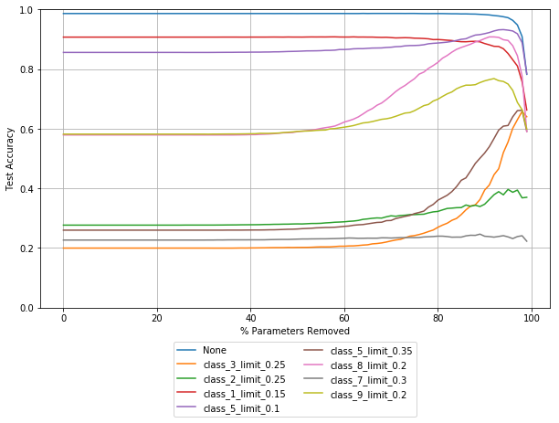
As you can see, robustness with respect to most of these noise vectors increases before any noticable drop in overall performance, which is shown as the top line in blue. Robustness with respect to some noise vectors stays relatively flat, or falls. Robustness with respect to some noise rises and the begins to fall while still rising for other noise vectors.
Activated Values
The plot below shows a 4 layer fully connected neural network pruned based on the smallest mean activated value.
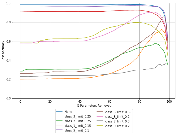
Overall performance (top line, in blue) begins to drop off sooner than absolute value pruning. Robustness with respect to all chosen noise vectors increases, but begins to fall in some cases while still increasing in others. There is no guarantee that other noise vectors will behave the same way, as seen in the variation between the plots here.
One interesting thing to note is that there are small step like improvements in in robustness for several noise vectors. This suggests that there are parameters that contribute only to adversarial corruption, but not to the overall performance of a model.
Combined performance
Here is a plot where both pruning techniques are used at the same time, Because of the earlier drop off in performance the parameters selected by activated values are pruned at 7% less than absolute value. So at 50% removed here the 50% of parameters with the smallest absolute value are removed, and 43% of parameters with the smallest activated value are removed.
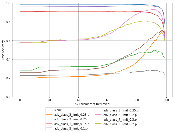
The majority of parameters removed by any point will have been removed by both methods, but the small ammount of parameters that are removed by one or the other results in slightly better robustness for some noise vectors.
Best Performance
Just for readability this is the best values that i got from some trial and error setting an arbitrary overall performance of 98.0%. The model is pruned at
Absolute values: 90%
Activated values: 81%
Combination prune: absolute values 85% and activated values 80%.
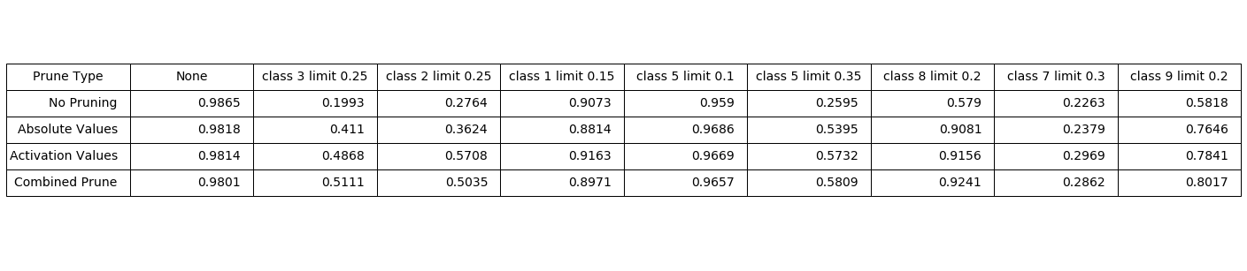
This shows that for this model, and these noise vectors pruning by activated values seems to have the best improvements in robustness. Combined pruning has some increases, and some decreases. Until there is are solutions for all adversarial additions, this shows that we can probably concentrate on dealing with some classes, or varieties of noise.
Pruning individual layers
The following plots show how models respond to having individual layers pruned, one at a time.
Absolute Values
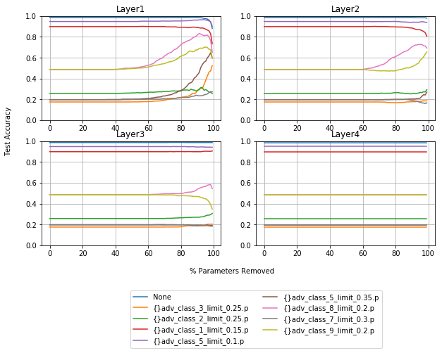
Activated Values
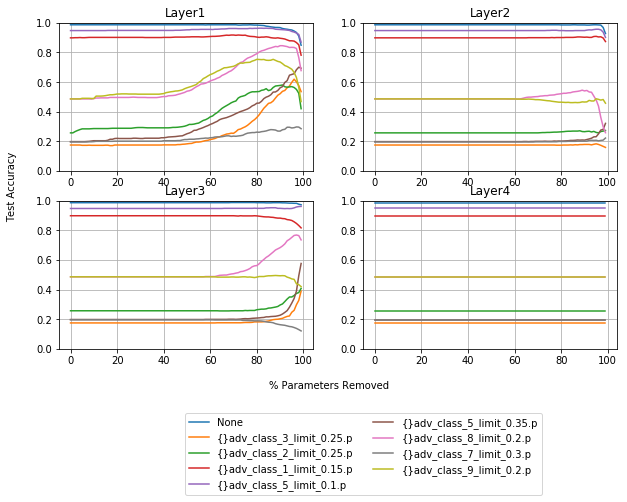
As you can see, the parameters that have the biggest influence when dealing with adversarial data, and performance in general, are the first layer. This may give some intuition about why logistic regression models are also prone to adversarial attacks.
Absolute value pruning has more increases in robustness in layer 2 than layer 3, and activated value pruning has more for layer 3 than layer 2. I have found this to be the case with other, similar models, and other noise vectors. This narrows down the step like improvements in robustness, mentioned earlier, to the first layer.
One thing that is worth mentioning is that in experiments pruning individual layers that they are not independent. The second and third layers can be pruned, in both instances by more than 95% without losing performance, but resiliance decreases. Overall performance starts to fall off much sooner when another layer is pruned.
CNN Pruning
Decoupled Convolutional Layers
Pruning fully connected networks show promising results, getting similar results with convolutional neural networks proved more difficult, with less impressive results. The fully connected networks shown above are pruned to be about 80%-90% sparse(80%-90% zero values). Convolutional layers are already equivalent to extremely sparse fully connected layers. I have converted the convlolutional layers of a trained network to see if pruning could have the same advantages. For small increases in robustness, overall accuracy decreases to similar point as the pruned fully connected model from above.
Tensorflow does not support the type of sparse operations, so for now, I have been using scipy sparse matrices for weight matrices. Operations are slow
While my results were not very promising, MNIST may not be the best dataset to work on, and pruning may well work better for other architectures. The architecture I have chosen is very simple, without even using pooling layers, which seem to have fallen out of favour. I will write another blog soon where I will concentrate more resources on improving robustness by pruning these layers.
Pruning fully connected layers
Pruning fully connected layers gets some increases in robustness, but the plots similar to the ones above are less useful. The first layer has many more parameters than the others, so pruning all layers by the same ratio does not work as well as the fully connected model. For this reason, I show only individual layer pruning, to choose the best combination of ratios for the chosen noise vectors.
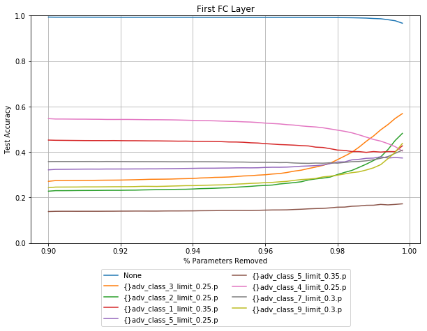
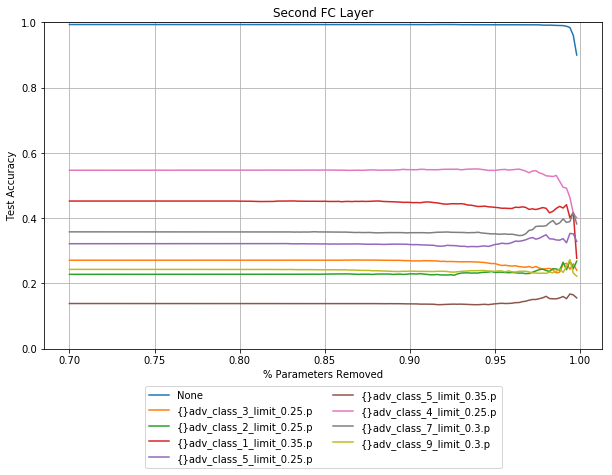
Activated value pruning
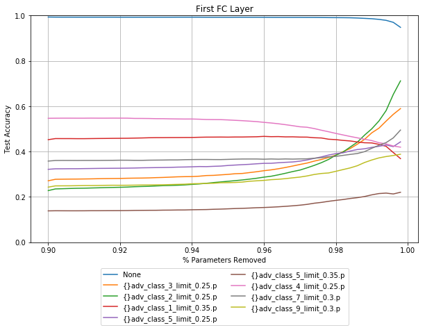
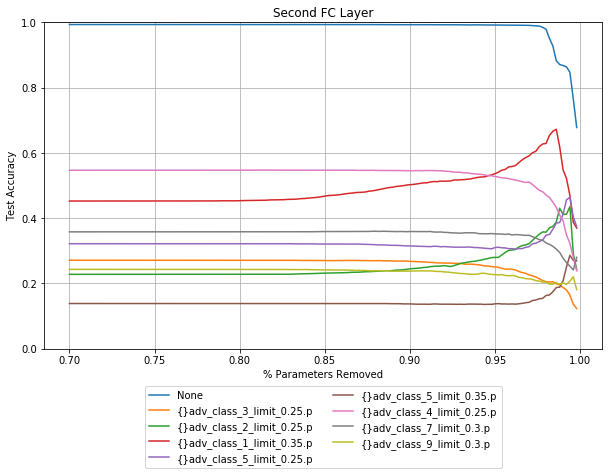
The X axis on these plots starts at 90% for the first layer, and 70% for the second layer. The inputs for the first fully connected layer are a the flattened final convolutinal layer, which in this case is 15680 activations. This means that this layer has far more weights than any other layer seen so far. Anyone familiar with the VGG networks will know that most of the parameters are in the first fully connected layer. Even by pruning 98% there is no drop in performance.
Similar to the fully connected networks, pruning different layers has a different effect with regards to different noise vectors. The accuracy for data corrupted by class 1 shown in red above, decreases when layer 1 is pruned, and increases when layer 2 is pruned.
Absolute value pruning
Activated value pruning was more effective in fully connected models, this seems to hold for CNNs, there are still some advantages to absolute value pruning for layer 1, pruning layer 2 has no robustness gain for these noise vectors.
While these plots don’t have the same robustness increase compared to the fully connected model pruning, the baselines start much higher. I have chosen the noise vectors here mostly at random, but have made sure to show that it is not all good news. Even in the fully connected models, there are noise vectors shown that can effectively attack a pruned model.
PARANA Package
I made a small package for building and pruning these models. It seemed easier than going though other peoples source code, and gave me a better understanding of everything. Also i am a cook, and self taught programmer, this was a bit of practice for me. The code is available on github, please excuse bad programming practices, and experimental dead ends that are in the code.
Conclusion and thoughts
It seems that pruning can improve robustness to some types of adversarial noise without losing overall performance. The methods used so far are agnostic to the type of noise, so should generalize quite well to other types of noise. Giving these methods an advantage to training a model to recognise specific types of noise. Getting machine learning models to perform as well on the benchmarks they achieve so far has been the culmination of many years of work with incremental improvements. The problem of adversarial noise is a complicated one that will likely be solved the same way.
This all shows that different types of noise interact with models in very different ways, solutions that work for one type of noise are not going to work for others.
In these cases pruning a fully connected model gives better improvements in robustness than pruning a convolutional model, which is effectively a very sparse fully connected model.
These methods are simple and easy to implement. No extra training time is needed for using the linear-quadratic cost method.
While these methods may be less effective than training a model on noise, there is an advantage to methods that are agnostic to the type of noise. Combatting adversarial noise using the noise that we know of quickly becomes unreallistic as new methods of producing the noise are discovered. If we can develop methods that are agnostic, we may be getting towards treating the problem that is inherent with these models to begin with.
Next Time
While robustness increases are less encoraging for CNNs than they are for fully connected ANNs, the next blog adds to the potential tools for dealing with adversarial noise. It looks at the outputs of linear-quadratic models in an attempt to detect which data has been corrupted.
Notebooks used:
- ANN pruning and visualisations: Generated the first plots pruning the whole network.
- ANN Layer pruning: Prunes individual layers, generated these plots
- CNN FC Layer pruning: Prunes the fully connected layers of convolutional neural networks
- Make_some_noise: generates noise for the fully connected models.
- CNNNOISE: generates the noise for CNNs
- CNN_DECOUPLE_PRUNING: decouples a CNN into fully connected sparse matrices, and prunes these models. These models are run in python, as of building this tensorflow did not support the type of sparse operation. Runs too slow to make plots from.
I have used these notebooks, but not as is. I have tried loading different models, pruning layers to different levels. I have removed the training loop cell from