Output analysis

In this blog I explain why I have chosen to remove the softmax function from the output. Then look at the output values to estimate a confidence value to indicate the quality of the input images. The confidence estimate value is then used to predict which inputs are corrupted by adversarial noise. Then I look at which images are more susceptable to adversarial corruption. This blog follows on from the previous one about techniques for pruning neural networks, which I have have used here. I would recommend reading throught that blog first.

Softmax-cross entropy vs. linear-quadratic

The standard technique for training a neural network is a cross entropy cost function applied to the softmax output of the final layer of the model. While other cost functions other than cross entropy are also used, the softmax is near universal. I have applied a quadratic cost function with L2 regularization to the outputs of the final layer. Without an activation function, this makes the final layer a linear function, hence the name linear-quadratic models. The model is clearly not a linear model, every other layer has ReLu activations. The justification for L2 regularization for linear models is that it reduces overfitting, this may or may not be the case, however I have found that it helps during training. Without L2 regularization, weights will often blow up, or decrease to 0 resulting in nonsensical outputs. This doesn’t seem to happen when using L2 regularization. I have found that models trained on MNIST achieve slightly higher test accuracy using the linear-quadratic method.

I showed in the last article that training adversarial noise is more difficult on a linear-quadratic model. I trained adversarial vectors by adding a softmax function to the final layer and using a cross entropy cost function. The noise trained is not a effective as using the same method on softmax-cross entropy models, but works well enough.

I have tried using ReLu outputs of the final layer, trained with quadratic cost, performance was similar, but would lead to undefined values for the 1-2 ratio mentioned below.

Output confidence measure 1-2 ratio

The optimization algorithm pushes the outputs to be equal to the one hot label vector of 0s and a 1. With sofmax-cross entropy this pushes the outputs before the softmax function to be in the range of -4 to 4, which will be close to 0s and a 1 after the softmax, this range can vary quite a lot depending on the model architecture. With linear-quadratic, the models outputs are very close to 1 and 0 without applying the softmax function.

I use a confidence estimate, which is the ratio of the highest value output divided by the second highest output. Looking at the output vectors, there are often 2 values that are similar in magnitude, and significantly bigger then the other values. Some intuition behind this is, when looking at some of the poorly written digits in MNIST, it is easy for a person to mistake a 2 for a 3, for example, but nobody will mistake it for a 1.

I want to be careful of refering to the outputs of a model as confidence, often there is no frame of reference. I have read articles refering to a 0.99 output of a softmax layer as 99% confidence with insifficient justification. Most researchers are also careful of this, but blogs and news sites are often guilty of this. The confidence estimate that i am using, is only useful in comparing an output to other outputs. The low confidence images below are only lower than the other images in the same sample set.

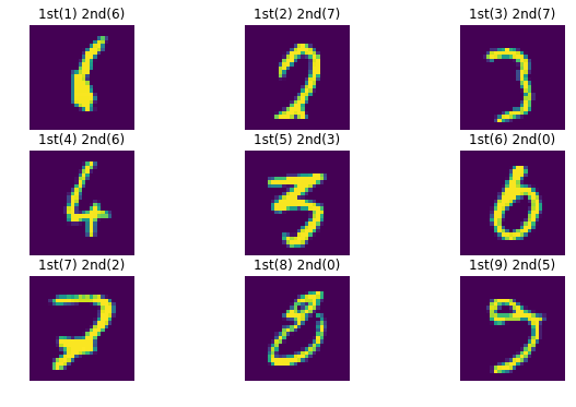
The images below show the correct class as 1st, and the class with the second highest value as 2nd.

Low Confidence Images

High Confidence Images

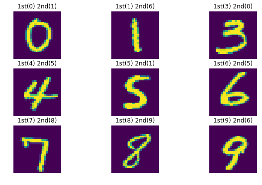
It seems obvious to me that the higher confidence images are better written, and clearer than low confidence images. It is also obvious how a model could mistake the highest (1st) for the second highest(2nd) in all of these images. I think that I would have mistaken the middle image for a 3 instead of a 5.

Some images with the highest confidence may not be the best handwriting, but are clearly not a different class. While I can see that a 3 has a big loop like a 0, the middle 5 and a 1 are about as dissimilar as any 2 digits could be. The second highest class value is still very low, hence these images having the highest confidence estimate values.

While I personally think that the higher confidence images are better written, I am clearly going to be biased towards wanting my own system to work. so the best way to test this scientifically would be to have people who have no particular bias to independently rate the images and see if human confidence lines up with these results.

MNIST is a good dataset for this exercize, because a person can look at an image and see why a digit could be one of 2 classes. For some of the images above, i can count how many pixels to change to change in the image, to probably change the class, just by looking. This becomes more difficult with bigger, more complex images and datasets, and may not work at all for other datasets.

For most images in MNIST that have a low confidence estimate there are 2 output values that are similar, but for a few low confidence images, there are more output values that are in a similar range.

Confidence and Adversarial Noise

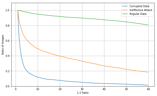
The reason for looking at this to begin with was to see if there was a clear distinction between clean, and corrupted data. Below is a plot of how many images have a 1-2 ratio below a given point. Half of the datapoints are corrupted with a randomly chosen noise vector of a different class. These are generated using the tensorflow MNIST test set, these images have not been used for training. Images from the training set have very similar results.

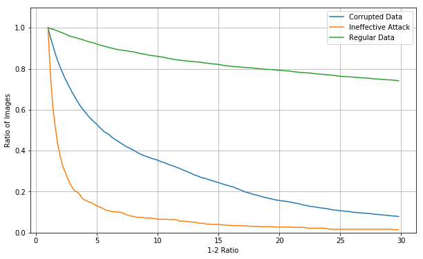
This is a cumulative distribution function, which shows how many values of a distribution are above or below a point. I think these are more practical than a histogram for visualising this data. The test accuracy for this set of 10,000 images without noise is 98.65%, and with noise added to 50% of images is 55.28%. 90% of clean images have a confidence estimate of above 6.6, and 44% of corrupted images do. 80% of clean images have a confidence estimate above 18.2 and 17.5% of corrupted images do.

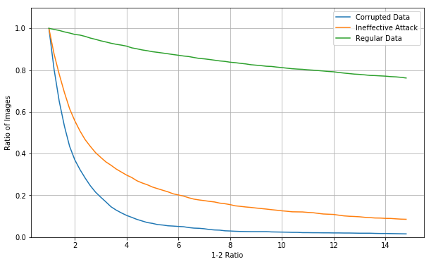
But how about a model that has been pruned like the last blog? This time the model has had 80% of its parameters removed based on the lowest mean activated value.

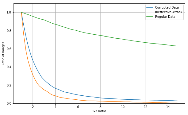
The overall accuracy for the test set is 98.28%, a slight drop, and the accuracy with noise added to 50% of images is 62.96%, which is a significant improvement, but not enough to really consider robust. The scale of the confidence estimate(X axis) here is different. The confidence value curve drops off for clean data faster for a pruned model than the original model. 90% of clean images have a confidence estimate value above 3.4, and 25% of corrupted images do. 80% of clean images have a confidence estimate above 7, and 9% of corrupted images do.

What about CNNs?

Convolutional neural networks behave in a simlar way, with most corrupted data having a low confidence estimate.

This model had a test accuracy of 99.3% and an accuracy with noise added to 50% of the datapoints is 76.89%, which is better performance than the unpruned fully connected network shown above. The scale of confidence values is much bigger for the CNN. Above I have chosen the arbitrary point of rejecting 10% of clean data, in that case, 5% of corrupted data would be effective as an attack.

As you can see, there are some corrupted datapoints that have a high 1-2 ratio.

Here is the 1-2 ratios from the same model after activation based pruning.

The performance with noise is slightly better, the 10% cutoff has the same 5% of effective corrupted data. There is less advantage of using a pruned CNN vs. un-pruned CNN compared to pruned fully connected network vs. unpruned fully connected network.

The noise vectors used for CNNs are less effective than those used for fully connected networks above, but this does show that there is a difference in confidence values.

Other Models

These plots are for the models that I have been using for all of these demonstrations. But there is quite a lot of variability found using different models. Training time and pruning rates have a big influence, and can lead to better or worse performance with reasonably small differences in test accuracy.

I have tested this with lower intensity noise vectors as well. The overall accuracy is better, but there seems to mostly be a small ammount of corrupted images that have high confidence estimates that can’t be effectively distinguished using this method.

Which images are susceptable to adversarial noise?

The lowest confidence images are more susceptable to adversarial attack, where the highest confidence images are more robust. Using the examples of the lowest and highest confidence images from above, I have corrupted the images with a noise vector of the same class as the second highest output. These values are from the unpruned fully connected network(first CDF plot). THe weak noise images have an epsilon values of 0.15, and the strong noise images have an epsilon value of 0.35 that is used in the rest of these demonstrations. First are the low confidence values.

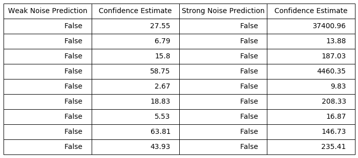
All of the images are corrupted by all of the noise vectors. Some of the weak noise images have confidence estimates in the lower range, but all of the strong noise outputs would fool any system.

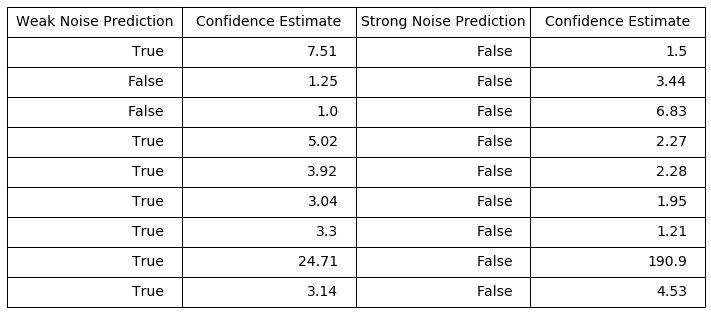
These images are much more robust, the weak noise vectors are not enough to corrupt 7 of these images, and the strong noise only corrupts the confidence by a large ammount in 1 case. This demonstration is not exhaustive, the next blog has more detailed tests of the effects of confidence on robustness.

Output values.

Here is a CDF of the maximum output values from the model. There is no regular data that has an output outside the range of 0.5-1.1, there are some corrupted inputs that have output values outside this range.

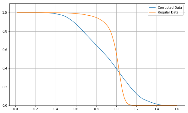
These outputs are for an unpruned, fully connected model. According to this plot, about 30% of outputs could be rejected for being outside an acceptable range. Unfortunately pruning moves the distribution of these outputs much closer together.

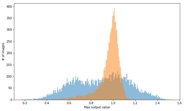
And because all of these values are in a similar range, here is a histogram of these distributions

I will include similar plots to these using CNNs and pruned models in the next blog.

Why the bigger range?

While it may be easy to generate noise with outputs in the same range as clean images, this noise is generated with a softmax function added. Models trained with the softmax function have a bigger output range, so it stands to reason that noise generated with the softmax function will also.

In Conclusion

Depending on how applicable this is to other models and datasets, these methods can go some way as to combatting potential adversarial noise. These methods can at least make adversarial attacks less worthwhile. If some of the most effective attacks can be made ineffective, and others have a high chance of being detected, attempting to use adversarial attacks maliciously has more risk and less reward.

All of these results are dependent on the type of noise being used. I am using only 1 type of noise for these articles. Testing on other types of noise will take a lot of time, especially as more types are generated, which may behave differently. I hope the results that I have shown are encoraging enought for others to try, the reason for the great things being achieved in this field is an open and colaborative environment, where researchers, and hobbyists (like me) can test and expand on existing work.

For many applications, rejecting legitimate, but low confidence datapoints is not a critical problem, a video input running many times a second could wait until the subject is close and clear, rejecting some images. Analysing the outputs should add very little overhead to a system using image, or in some cases could be more efficient, if the result leads to no further action being taken.

I have tried to avoid speculation in these blogs, focusing more on results. I will write more of my thoughts about how and why these methods work in a later blog.

Notebooks used

output analysis: Fully connected model output analysis
CNN output analysis: Convolutional neural network output analysis

jngannon.github.io